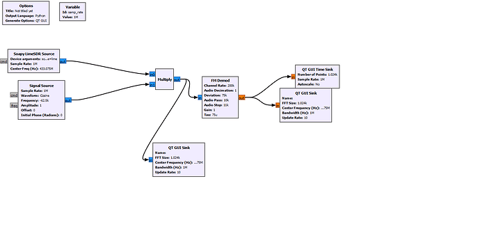
why is it that when I receive a frequency modulated signal (without demodulation), its parameters decrease by 2 times
please can I have a detailed description of why this is happening
Your demod block looks suspect - you don’t have the correct sample rate set for it. Also, such a block has filtering for the de-emphasis, and that will limit your demod.
Also, what are the settings for the Lime on RX? Do you perhaps have too narrow a front-end filter setting and/or too narrow an IF filter setting?
This graphical interface costs UP TO demodulation, the signal comes to the receiver half as much at once. RF and TX Gain are both at 40db, BW=samp_rate=1M. FM demod gives an error when setting a high sampling rate
It is not clear what you are trying to, but the example " FMLime04qt.grc" at
captures and plays the local FM stations. It can be converted to receive many types of FM signals.
I noticed that you are doing a complex to real before the frequency sink in the generation path, and are directly plotting the complex signal in the receive path. Try changing the plot on the generate side to a complex frequency sink, and bypassing the complex to real, and see if your data matches.
Thank you, it helped a little, but for some reason it eats 30db from the bottom, when transmitting the signal goes up to 150 dB somewhere, and when receiving up to 120.
Don’t rely upon the absolute levels reported by these sorts of graphs. Without calibration on the RX path the absolute values are meaningless. And on the TX path, unless you define some sort of relationship between the arbitrary numbers used in the data and the actual RF levels, again the absolute values are meaningless. You would have to have some guaranteed, calibrated relationship between 0dB full scale on the data path and 0dBmW on the transmitter, which will be a function of TX gain, any filters on the TX output, any gain elements on the TX, etc.
Trust me - I design SDR test instruments for a living. Getting the calibration right is the single biggest part of what differentiates a two hundred dollar “gizmo to play with” and a sixty thousand dollar lab grade test instrument.
When you go to the complex plot on TX, do you see the same width of signal as on RX? Do you see roughly the same spectrum?
Yes, the spectrum is the same. I am doing a term paper on this topic and the teacher told me to explain why these 30 dB disappear from the bottom. Is there any way to calibrate these values? He said that you can leave it like that, but you need to explain in detail why this is happening and I can’t write “just don’t pay attention” ![]()
Well, I think I’d like to see a picture of your plot so I can better understand what you mean by “30 dB disappear”. It could be simply that you don’t have the plot scales set correctly, and that if you adjust the vertical offset of the scale you might see what you expect.
As for calibrating the scales… First, consider the generate side of things. Until you get to the actual hardware, you aren’t dealing with physical values, just numbers. How many volts is .707 - .707i ? The answer is “whatever you define it to be.” The only thing you can do is work in terms of dBfs - decibels relative to full scale. In other words, you say that a sinusoid going from -1.0 to 1.0 (for a floating point signal) is full scale, and thus is a 0 dBfs signal. (if you are working in integer type values, like a 16 bit int, then you would use -32767 to 32767 as your full scale value).
So, then you have to define the transfer function of the transceiver from input data to output voltage. You are going to have to define a specific gain value, e.g. maximum gain, and then what you expect the output level to be for a 0dBfs signal. Of course, the nature of that signal will impact the levels - if you feed a steady 1+0i signal in that is going to be a different level output than if you feed in a sinusoid at just under half the sample rate, due to the response curve of the transceiver. So, you make a statement like “I will define that the transfer function of the transceiver shall be 0dBfs in at center frequency shall be 20dBm + 10log10(gain setting/50)” (that 50 being some constant for the hardware’s gain control, and of course assuming the gain setting is linear, not already logarithmic.) And making that statement be true usually requires a LOT of time in a lab, with a lab grade measuring receiver.
Continuing on, then there is the receive path. Again, you have to define a transfer function between the input of the receiver hardware and the data stream. It gets tricky, because you have things like the gain control of the receiver, the losses of any roofing filters on the front end of the receiver, any filters in the receiver hardware (both analog filters and any digital filters), any gain due to decimation. And if you are using hardware based automatic gain control, then you have to have some way to capture the gain that was used when a block of samples were captured so that you can apply that to the transfer function. And again, the frequency response of the channel plays into that - for example, most ADCs have a sinc(f) type frequency response, so that as you get to the edges of the passband, the gain goes down. If you are actually doing measurements, you have to apply a 1/sinc(f) compensation somewhere in the processing, either in the digital filters in the hardware or in a filter in the processing chain. And again, making that conversion actually be accurate takes a lot of time with lab grade signal generators, attenuating pads, power splitters, measuring receivers, and a high frustration tolerance.
And then there are all the fun bits like temperature compensation, drift over time, and that damn cable that should have been thrown in the trash because it has a bad connection in one end and some corrosion on the center pin.
That’s why I counsel just working in relative values - you can talk about the levels of the different parts of the spectrum vs. the carrier signal, or vs. 0dBfs, or relative each other, and you will probably be OK. On the RX path, one thing you can to is put a software AGC block in that can be enabled or frozen. Enable it, feed a dead carrier into the TX side (again, 1+0i for all samples), and let the AGC block servo the signal to 0dBfs (alternatively, use a manually controlled gain block and adjust it yourself). Then you freeze the AGC and you should be able to compare your signals a bit better.
OR - just accept that the top of scale on RX plots does not map to any specific top of scale on the TX path, and only the relationships within the graph matter. You then adjust the top of scale for the plots to get the signal in roughly the same place on each plot (keeping the width of the plots and the height of the plot in terms of (top of scale)-(bottom of scale) the same).
If you want some more information on some of the fun bits, here’s a like to a standards definition organization I belong to and some of the standards I helped author:
https://sds.wirelessinnovation.org/specifications-and-recommendations
Including the transceiver specification that I was one of the lead contributors to:
https://winnf.memberclicks.net/assets/work_products/Specifications/WINNF-TS-0008-V2.1.1-all-volumes.zip
Unfortunately, I won’t be able to do it again until May 10, because the equipment is at the university. If you don’t lost this discussion, I’ll send it to you.
Thank you, I will try to read and delve deeper into this topic
Looking at that plot and the plot of what you received, I think you are getting a reasonable match other than the fact that the RX is low because you are not getting enough signal into the hardware. In your RX plot you only have 40dB of dynamic range due to the low signal level, while your new TX plot has 150dB of dynamic range.
You need more power into the RX. Are you using a cable between the TX and RX, or are you using 2 antennas? If you are using antennas, you need to increase the gain on the RX by at least 30 dB so that you can get at least 70dB of dynamic range. If you do that, you will see more of your side lobes, and your RX will start to look more like your TX.
It would also help to set your widths to match on the two plots, just to make comparing them with the Mark 1a eyeball diff a lot easier.
Thanks for the reply, I am using two Lime SDRs. I transmit using one computer and Lime SDR and receive on another.
Also, as I said earlier, the transmit and receive gain is 40dB. Could the problem be that the graphical interface just shows the generated signal, which only then goes to transmission? Because after the transfer it is impossible to put the GUI to see.
It’s not the GUI per se. It’s that you don’t have enough signal on the receiving device. Looking at the levels you show, I suspect you are not connecting the devices with a cable; you are using 2 antennas, right? If so, you don’t have enough coupling to get a strong signal on the receiving device - either you don’t have enough TX power, or you don’t have the antennas close enough together. Use a coaxial cable between the transmitting device’s TX out and the receiving device’s RX in, and you will get enough signal level to see your signal in all its glory.
Thanks again for your reply. Yes, I use 2 antennas. I won’t bother so much, I’ll just write as you said)


